Implementation

The algorithm computes a normalized volume (between 0 and 1), and is roughly split into 4 steps:

1. Compute a tessellation
2. Compute side-length values
3. Trim simplices
4. Compute the normalization

Compute a Tessellation

After integrating an orbit, the raw point-array of its position over time is passed into a tessellation algorithm. For this specific implementation, SciPy's Delaunay Tessellation routine is used, which itself calls out to Qhull under-the-hood.

Compute Side-Length Values

The important values to compute here are the smallest side-lengths and longest side-lengths of the simplices in our tessellation. These are what will be used in our trimming condition.

Trim Simplices

The median of the smallest simplex side-lengths probes the length-scale of "related" parts of an orbit. If the longest side of a simplex is significantly larger than this value, it likely connects unrelated parts of the orbit and should be trimmed.

This threshold is referred to as the axis ratio, and is set to 10 by default. The trimming condition can be written out as so:

\[ \frac{\text{longest side}}{\text{median(all shortest sides)}} > \text{axis ratio} \]

05101520

100×100 example image of a slice of phase space. All simplices with an axis ratio above 0 are removed. Commensurability is calculated from the remaining simplices.

No Total Measure

By setting the axis ratio threshold to 0, all simplices are removed.

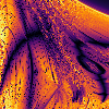
100×100 example image of a slice of phase space. All simplices with an axis ratio above 5 are removed. Commensurability is calculated from the remaining simplices.

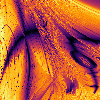
100×100 example image of a slice of phase space. All simplices with an axis ratio above 10 are removed. Commensurability is calculated from the remaining simplices.

This is the default.

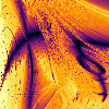
100×100 example image of a slice of phase space. All simplices with an axis ratio above 15 are removed. Commensurability is calculated from the remaining simplices.

100×100 example image of a slice of phase space. All simplices with an axis ratio above 20 are removed. Commensurability is calculated from the remaining simplices.

Compute the Normalization

There is some delicacy in choosing an appropriate normalization. The canonical choice is a hypersphere that encapsulates the whole orbit, but orbits rarely fill a whole hypersphere, resulting in poor dynamic range.

In 2D, the default normalization a circle that encapsulates the orbit (routine name is circle). This is the only normalization routine available.

In 3D, the default normalization takes 4 rotated copies of the point array and computes its convex hull (routine name is convexhull_rot4).

Normalization Routines in 3D

SphereCylinderConvex HullConvex Hull in \(R\) vs \(z\)4 Rotated Convex Hulls

100×100 example image of a slice of phase space generated with sphere normalization. Normalizing shape is the smallest enclosing sphere centered at the origin.

100×100 example image of a slice of phase space generated with cylinder normalization. Normalizing shape is the smallest enclosing cylinder centered at the origin.

100×100 example image of a slice of phase space generated with convexhull normalization. Normalizing shape is the convex hull of the points.

Co-rotation Tracks

Co-rotation resonance tracks are difficult to detect with this normalization routine.

100×100 example image of a slice of phase space generated with Rz_convexhull normalization. Normalizing shape is the convex hull in the \(R\) vs \(z\) plane rotated about the \(z\)-axis.

100×100 example image of a slice of phase space generated with convexhull_rot4 normalization. Normalizing shape is the convex hull of 4 rotated copies of the points about the \(z\)-axis.

This is the default.