Commensurability Quickstart

commensurability is a package that provides tools for analyzing commensurabilities within galactic potentials. It contains subpackages that implement particular algorithms for evaluating an orbit's commensurability.

Installation

See installation for full installation details.

pip install commensurability

Usage

Galactic Dynamics Setup

This package is compatible with the galactic dynamics packages agama, gala, and galpy. To get started, set up a function that defines and returns a particular galactic potential:

AgamaGalaGalpy

def potential_definition():
    import agama

    bar_pot = dict(
        type="Ferrers",
        mass=1e9,
        scaleRadius=1.0,
        axisRatioY=0.5,
        axisratioz=0.4,
        cutoffStrength=2.0,
        patternSpeed=30,
    )
    disk_pot = dict(type="Disk", mass=5e10, scaleRadius=3, scaleHeight=0.4)
    bulge_pot = dict(type="Sersic", mass=1e10, scaleRadius=1, axisRatioZ=0.6)
    halo_pot = dict(type="NFW", mass=1e12, scaleRadius=20, axisRatioZ=0.8)
    pot = agama.Potential(disk_pot, bulge_pot, halo_pot, bar_pot)
    return pot

import astropy.units as u

def potential_definition():
    import gala.potential as gp
    from gala.units import galactic

    disk = gp.MiyamotoNagaiPotential(m=6e10 * u.Msun, a=3.5 * u.kpc, b=280 * u.pc, units=galactic)
    halo = gp.NFWPotential(m=6e11 * u.Msun, r_s=20.0 * u.kpc, units=galactic)
    bar = gp.LongMuraliBarPotential(
        m=1e10 * u.Msun,
        a=4 * u.kpc,
        b=0.8 * u.kpc,
        c=0.25 * u.kpc,
        alpha=25 * u.degree,
        units=galactic,
    )
    pot = gp.CCompositePotential()
    pot["disk"] = disk
    pot["halo"] = halo
    pot["bar"] = bar
    return pot

import astropy.units as u

def potential_definition():
    import galpy.potential as gp

    omega = 30 * u.km / u.s / u.kpc
    halo = gp.NFWPotential(conc=10, mvir=1)
    disc = gp.MiyamotoNagaiPotential(amp=5e10 * u.solMass, a=3 * u.kpc, b=0.1 * u.kpc)
    bar = gp.SoftenedNeedleBarPotential(
        amp=1e9 * u.solMass, a=1.5 * u.kpc, b=0 * u.kpc, c=0.5 * u.kpc, omegab=omega
    )
    pot = [halo, disc, bar]
    gp.turn_physical_on(pot)  # ensure Astropy units support
    return pot

Why define a separate function? When writing a commensurability analysis object to disk, this function's source is stored along with the generated data. This way, the potential can be reconstructed when reading data back into an analysis object, allowing for continued analysis within the same potential.

After defining a potential, we must define a region of phase space to probe for commensurate orbits.

Initial Conditions

The region of phase space is specified by two arguments:

• an "initial condition" function that returns a astropy.coordinates.SkyCoord object.
• a dictionary of sequences of values to be passed into the "initial condition" function, defining the dimensions of the data to be generated.

Suppose we want to explore orbits starting between 2 and 8 kiloparsecs with an initial tangential velocity between 200 and 300 kilometers per second, starting 2 to 4 kiloparsecs above the galactic plane. A 30x30x5 data cube for this region in phase space can be defined as follows.

import astropy.coordinates as c
import astropy.units as u
import numpy as np

def initial_condition(x, vy, z):
    return c.SkyCoord(
        x=x * u.kpc,
        y=0 * u.kpc,
        z=z * u.kpc,
        v_x=0 * u.km / u.s,
        v_y=vy * u.km / u.s,
        v_z=0 * u.km / u.s,
        frame="galactocentric",
        representation_type="cartesian",
    )

values = dict(
    x=np.linspace(2, 8, 20),
    vy=np.linspace(200, 300, 20),
    z=np.linspace(2, 4, 5),
)

Lastly, the simulation parameters must be defined, namely the time step and number of steps.

dt = 0.01 * u.Gyr
steps = 1000

Running Analysis

This region of phase space can be probed for commensurabilities using one of the Analysis classes provided in the commensurability package.

from commensurability import TessellationAnalysis

Collecting everything, we can pass the above objects in the following order:

# tessellation needs to know the pattern speed used to define the potential
# so that it can perform its analysis in the co-rotating frame
omega = 30 * u.km / u.s / u.kpc
tanal = TessellationAnalysis(initial_condition, values, potential_definition,
                             dt, steps, pattern_speed=omega)

This step will take a while. Once this is done, it is recommended to write the object to disk—the object is fully recoverable from the disk. All analysis objects are stored using the HDF5 format.

# to save to disk
tanal.save("example_analysis.hdf5")

# to read from disk
tanal = TessellationAnalysis.read_from_hdf5("example_analysis.hdf5")

Launch an Interactive Plot

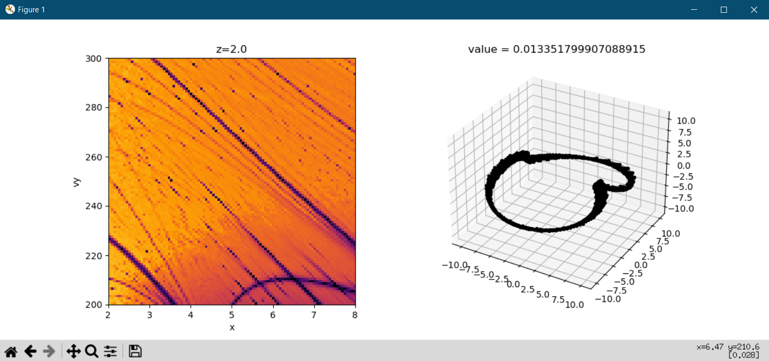
Analysis objects can launch interactive plots to explore the generated data. Currently, interactive plots work with up to 3 dimensions of the generated data. Specify two variables for the plotting axes, and optionally specify a third to vary using the scroll wheel. For 3 dimensional data, the scroll wheel varies the remaining variable by default.

tanal.launch_interactive_plot()

This should launch a window with two plots side by side: the left is a visualization of the commensurability data within phase space, and the right will display integrated orbits. A left-click in the left plot will generate the corresponding orbit from that initial condition. A right-click in the left plot will do the same, but also compute and visualize a commensurability evaluation.

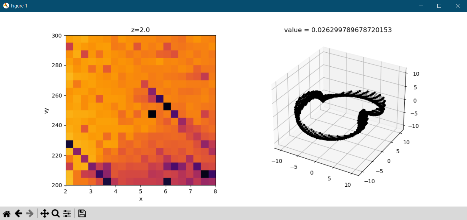
Running this example for a finer grid size produces the following plot: